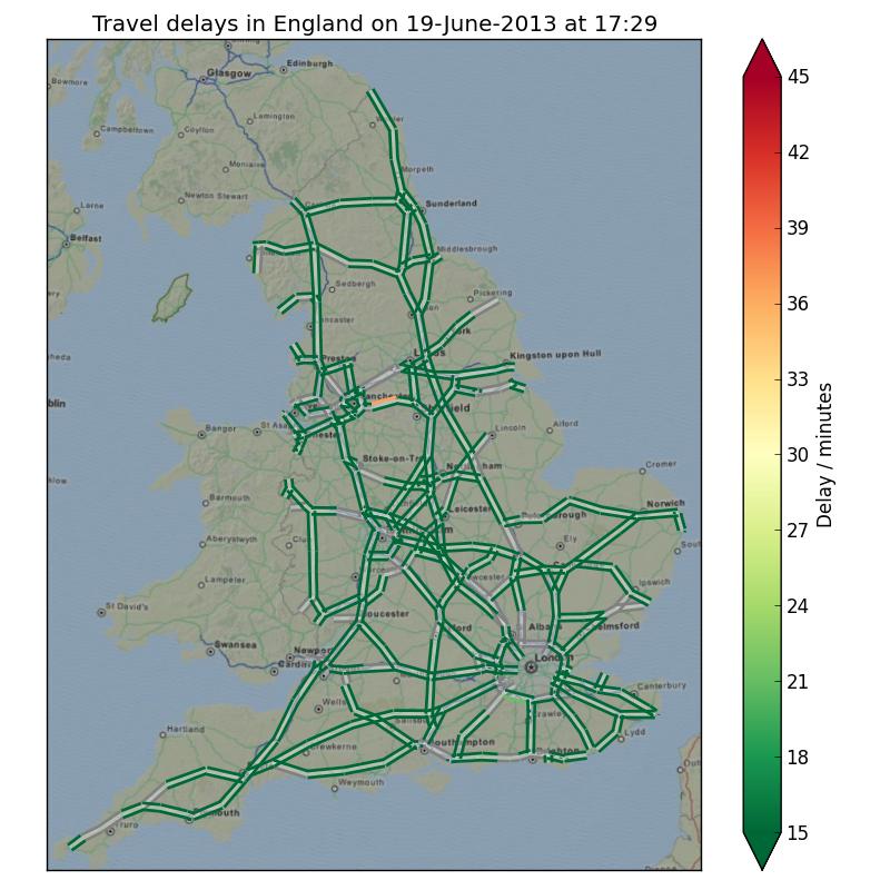
In this post: parsing the real-time traffic feed from the UK Highways Agency; plotting the UK's major road links an map using the Ordinance Survey national grid; colouring the result nicely.
The UK Government's data.gov.uk website is a treasure-trove of data just waiting to be downloaded. Recently I started some pre-research on a project at work to do with traffic congestion prediction for which getting some actual historical data on the state of the roads in the UK would be useful. Luckily the data.gov.uk website has a section on live data from the UK Highways Agency. I decided it would be useful to play with this data and see what I could get out of it.
What is available
The data itself takes the form of XML documents which are updated every so often with the current state of the road network in England. Some files are updated around once every 10 minutes. For example, the UK Highways Agency maintain a network of Automatic number plate recognition systems which measure journey times along major links in the UK's road network. It uses this information to publish three bits of data about each link:
- the current journey time;
- the typical journey time; and
- the ideal journey time in free-flowing traffic.
It is such data which is used to create traffic delay maps such as the one at the top of this post or elsewhere online.
Road locations
According to data.gov.uk, the location data for journey time data is available from the following URL:
http://hatrafficinfo.dft.gov.uk/feeds/datex/England/PredefinedLocationJourneyTimeSections/content.xml
This document defines a list of locations which, for journey times, are starting and ending points. If we join a line from the start point to the end point for each location we'll end up with a crude road-map of England. There is a corresponding document which describes the schema for this XML document but, for our purposes, it is sufficient to look at a single truncated and annotated example. I've left out elements which we wont be using.
<d2LogicalModel xmlns="http://datex2.eu/schema/1_0/1_0" modelBaseVersion="1.0">
  <payloadPublication xmlns:xsi="http://www.w3.org/2001/XMLSchema-instance"
    xsi:type="PredefinedLocationsPublication" lang="en">

    <!-- An ISO8601 date for the data -->
    <publicationTime>2013-06-12T11:59:15+01:00</publicationTime>

    <!-- This set of locations is for journey time data -->
    <predefinedLocationSet id="GUID-NTCC-JourneyTimeSections">

      <!-- There is one predefinedLocation element for each section of road -->
      <predefinedLocation id="Section11017">

        <!-- The road location: a line segment joining a 'from' point to a 'to' point -->
        <predefinedLocation xsi:type="Linear">
          <tpeglinearLocation>

            <to xsi:type="TPEGNonJunctionPoint">
              <pointCoordinates>
                <latitude>52.51527</latitude>
                <longitude>-1.725507</longitude>
              </pointCoordinates>
            </to>

            <from xsi:type="TPEGJunction">
              <pointCoordinates>
                <latitude>52.54374</latitude>
                <longitude>-1.721629</longitude>
              </pointCoordinates>
            </from>

          </tpeglinearLocation>
        </predefinedLocation>
      </predefinedLocation>
    </predefinedLocationSet>
  </payloadPublication>
</d2LogicalModel>
Parsing
Fetching and parsing this document is the work of a few lines thanks to the Python standard library and lxml's
objectify module:
from lxml.objectify import parse
from urllib2 import urlopen

locations_root = parse(urlopen(PREDEFINED_LOCATIONS_DOCUMENT_URL)).getroot()
Here I've assumed that you've set the value of PREDEFINED_LOCATIONS_DOCUMENT_URL to the URL referenced above. (If
you're using Python 3, the urlopen function has moved into the urllib.request package.) The objectify module makes
the contents of the XML file available as attributes on the object. For example, we can get the publication time for the
document in one line. Using the iso8601 package, we can parse it into a standard Python datetime object:
>>> print(journey_time_root.payloadPublication.publicationTime.text)
2013-06-19T14:30:00+01:00
>>> import iso8601
>>> pub_time = iso8601.parse_date(journey_time_root.payloadPublication.publicationTime.text)
>>> print(repr(pub_time))
datetime.datetime(2013, 6, 19, 14, 30, tzinfo=<FixedOffset '+01:00'>)
>>> print(pub_time)
2013-06-19 14:30:00+01:00
The objectify module also exposes lists of elements via a standard Python iterator and so getting a list of all
locations a one-liner:
locations = list(locations_root.payloadPublication.predefinedLocationSet.predefinedLocation)
We can now easily extract the 'to' and 'from' points for each location. For example, the 'to' element for the location at index 10 can be pulled out in one print statement:
>>> to_coord = locations[10].predefinedLocation.tpeglinearLocation.to.pointCoordinates
>>> print(tostring(to_coord, pretty_print=True))
<pointCoordinates xmlns="http://datex2.eu/schema/1_0/1_0" xmlns:xsi="http://www.w3.org/2001/XMLSchema-instance">
  <latitude>52.51759</latitude>
  <longitude>-1.726274</longitude>
</pointCoordinates>
We can do the same with the 'from' co-ordinate but note that we have to use a different way to select the 'from' element
since from is a reserved word in Python:
>>> from_coord = locations[10].predefinedLocation.tpeglinearLocation['from'].pointCoordinates
>>> print(tostring(from_coord, pretty_print=True))
<pointCoordinates xmlns="http://datex2.eu/schema/1_0/1_0" xmlns:xsi="http://www.w3.org/2001/XMLSchema-instance">
  <latitude>52.49218</latitude>
  <longitude>-1.715665</longitude>
</pointCoordinates>
So, putting it all together, we can write a little helper function which will, given a predefinedLocation element,
return a pair of longitude, latitude pairs which we can use for plotting later on:
def location_to_lnglat_pair(location):
    to = location.predefinedLocation.tpeglinearLocation.to
    from_ = location.predefinedLocation.tpeglinearLocation['from']
    to_lnglat = (float(to.pointCoordinates.longitude), float(to.pointCoordinates.latitude))
    from_lnglat = (float(from_.pointCoordinates.longitude), float(from_.pointCoordinates.latitude))
    return (to_lnglat, from_lnglat)
We now have a way to get both the location start and end points and also the location's 'id'. This latter value will be important later on when we want to work out what the current delay is for a particular location.
>>> print(location_to_lnglat_pair(locations[10]))
((-1.726274, 52.51759), (-1.715665, 52.49218))
>>> print(locations[10].attrib['id'])
Section10976
Let's arrange the locations into a dictionary. The keys of the dictionary will be the location 'id's and the values will be the start and end points.
location_segments = dict((l.attrib['id'], location_to_lnglat_pair(l)) for l in locations)
Plotting
The matplotlib library has a handy LineCollection object which can be used to directly plot a set of linear segments in very few lines:
from matplotlib.pyplt import *
from matplotlib.collections import LineCollection

lc = LineCollection(location_segments.values())
gca().add_collection(lc)
axis('equal')
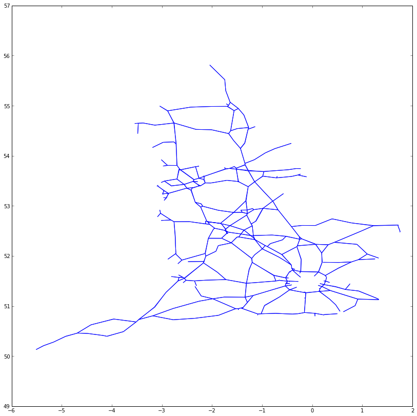
The road network is recognisable there but England appears squashed. That's because the co-ordinates are latitudes and longitudes. Using these directly to plot a graph is something called the equirectangular projection. This projection isn't usually used for maps of the British Isles since, at our latitude, the projection artifically 'widens' maps making them look too short and fat. To combat that, maps of England tend to use the Ordinance Survey National Grid. This projection has the advantage of, around England, low distortion and it corresponds to metres East and North of an origin somewhere off the coast at Land's End.
Most common map projections have an 'EPSG' code associated with them. For example, the direct use of latitudes and longitudes is EPSG:4326 and the Ordinance Survey National Grid is EPSG:27700. The Python GDAL library can be used to convert between them:
from osgeo import osr

bng = osr.SpatialReference()
bng.ImportFromEPSG(27700)

wgs84 = osr.SpatialReference()
wgs84.ImportFromEPSG(4326)

wgs84_to_bng = osr.CoordinateTransformation(wgs84, bng)
We can convert a location's to and from point to the National Grid using the TransformPoints method:
>>> print(wgs84_to_bng.TransformPoints(location_segments.values()[10]))
[(348854.1132332537, 309682.47213134286, -50.45861489698291), (369860.10673155746, 309570.42095603154,
-50.11469571758062)]
Notice that there is a third co-ordinate returned. This corresponds to the height of the point. We won't use this for our map and so we'll write a little helper function which strips it off:
def segment_to_bng(segment):
    return list(x[:2] for x in wgs84_to_bng.TransformPoints(segment))
Now we can convert a segment straight into the National Grid co-ordinates:
>>> print(segment_to_bng(location_segments.values()[10]))
[(348854.1132332537, 309682.47213134286), (369860.10673155746, 309570.42095603154)]
Let's use this function to generate a NumPy array object whose rows correspond to location segments:
>>> import numpy as np
>>> segment_coords = np.array(
...   list(segment_to_bng(location_segments[loc]) for loc in location_ids)
... )
>>> print(segment_coords[9:12,:])
[[[ 374985.14188095  399376.78814614]
  [ 376710.14637564  403171.80369787]]

 [[ 348854.11323325  309682.47213134]
  [ 369860.10673156  309570.42095603]]

 [[ 392143.39283833  304499.91516244]
  [ 396831.4499708   303504.82102035]]]
Using NumPy's slicing syntax, therefore, the co-ordinates of the 'to' point for the location at index 7 will be
segment_coords[7,0,:] whereas those for the 'from' point for the location at index 10 will be
segment_coords[10,1,:]. The array itself has three axes:
>>> print segment_coords.shape
(871, 2, 2)
We can plot these new segments as before:
lc = LineCollection(segment_coords)
gca().add_collection(lc)
axis('equal')
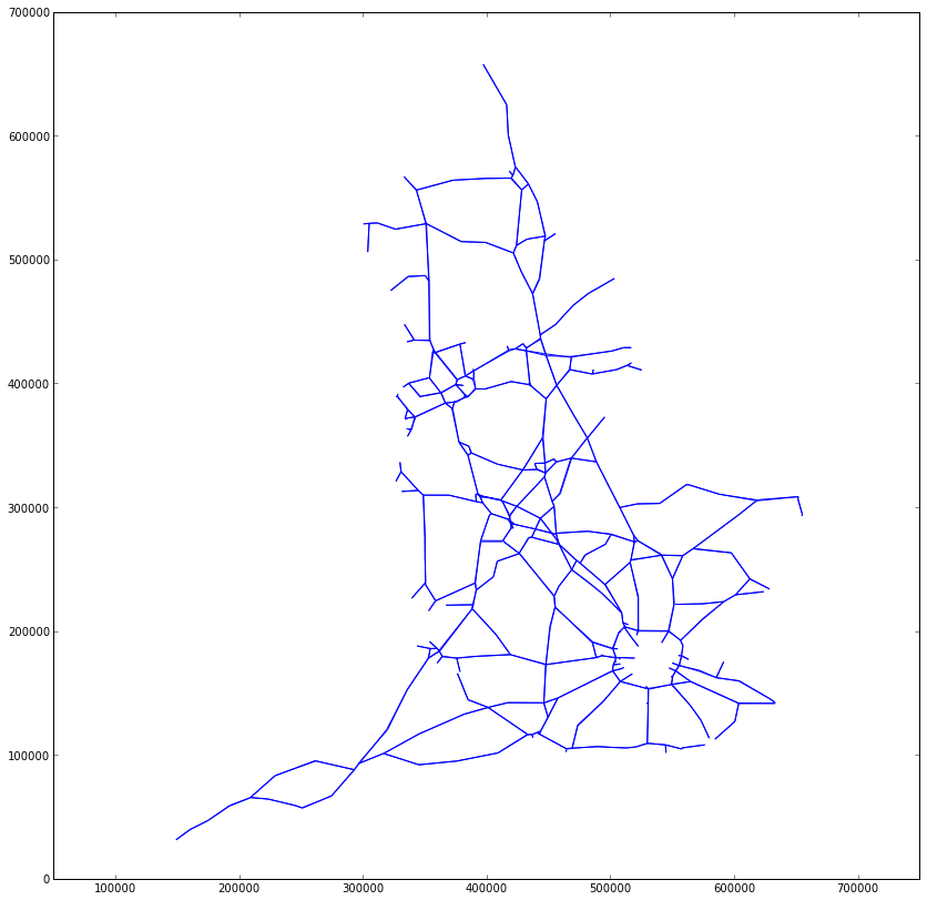
Notice how the distortion of England is now reduced and, also, that the plot's x- and y-axes are now in metres.
Adding a base map underlay
It would be nice to get a base map under the road network so that we can orient ourselves with respect to major cities
and the coastline of England. The GeoTIFF format is a variant of the TIFF image
format which can contain information about projection and geographic boundaries. Using my foldbeam tool, I've
generated a suitable GeoTIFF which can be downloaded from this
website. The GDAL library can also be used to load this image. I'll assume you've downloaded it to a directory and set
the DOWNLOADS_DIR variable to the path of that directory. Opening the base map image is then very simple indeed:
import os
from osgeo import gdal

# DOWNLOADS_DIR is the location of your downloads folder
base_map_ds = gdal.Open(os.path.join(DOWNLOADS_DIR, 'england-basemap-osgrid.tiff'))
The advantage of the GeoTIFF format is that it has encoded within it the numbers required to let us transform between pixel co-ordinates and projection co-ordinates, in this case the OS National Grid:
>>> print(base_map_ds.GetGeoTransform())
(130000.0, 671.2158808933002, 0.0, 700000.0, 0.0, -670.8984375)
We're going to use matplotlib's imshow function to plot the image. This function takes an extent parameter which
describes the minimum and maximum x- and y-co-ordinate for the image. We can calculate this from the numbers stored in
the GeoTIFF:
origin_x, pixel_size_x, _, origin_y, _, pixel_size_y = base_map_ds.GetGeoTransform()

# Compute minx, maxx, miny, maxy for image. Notice that, since pixel_size_y is -ve, the miny is not origin_y.
base_map_extent = (
    origin_x, origin_x + pixel_size_x * base_map_ds.RasterXSize,
    origin_y + pixel_size_y * base_map_ds.RasterYSize, origin_y,
)
An annoying wrinkle is that the imshow function expects a NumPy three-axis array with the red, green and blue
components of the pixel along the last axis. As you can see, the GeoTIFF format has the red, green, blue and alpha
channel information running along the first axis:
>>> base_map_ds.ReadAsArray().shape
(4, 1024, 806)
To fix that we use NumPy's transpose function. Plotting the roads atop the base map is then very simple indeed.
base_map = np.transpose(base_map_ds.ReadAsArray(), (1,2,0))
imshow(base_map, extent=base_map_extent)
lc = LineCollection(segment_coords)
gca().add_collection(lc)
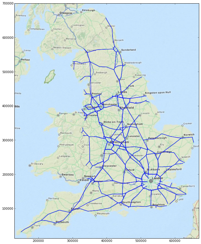
Offsetting each carriageway
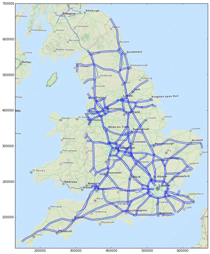
It isn't obvious from the map above but each link is actually defined twice, once for each carriage way. The difference is in the ordering of the 'to' and 'from' points. Traffic maps usually offset each carriage way so that both may be seen. The carriageway is offset, subjectively, to the left since that is the side of the road that we drive on here in the UK. Although we specify the co-ordinates of each line segment in OS National Grid co-ordinates, we'd like to specify the offset in figure co-ordinates. These will be either points or pixels depending on the matplotlib backend in use. Before we can construct a set of 'left' directions for each segment, we need to work out the direction of each segment. This is simply the 'from' point subtracted from the 'to' point. We also need to normalise these directions to unit length:
# Compute unit direction of each segment
segment_directions = segment_coords[:,1,:] - segment_coords[:,0,:]
segment_directions /= np.sqrt((segment_directions ** 2).sum(-1))[..., np.newaxis]
The normalising one-liner is a good one to remember here. Once we have a vector pointing along the segment, 'left' is just this vector rotated 90 degrees anticlockwise. If you remember your high-school geometry, a rotation anticlockwise by $\theta$ radians can be represented as a multiplication by a matrix:
$$ \begin{bmatrix} x' \\ y' \end{bmatrix} = \begin{bmatrix} \cos \theta & - \sin \theta \\ \sin \theta & \cos \theta \end{bmatrix} \begin{bmatrix} x \\ y \end{bmatrix} $$
Since, for a 90 degree rotation, $\cos \theta = 0$ and $\sin \theta = 1$, computing the 'left' vectors is actually fairly straight-forward:
segment_offsets = segment_directions.dot(np.array([[0, -1], [1, 0]]))
Now we've got these offsets, plotting each segment offset by, in this example, 2 points to the left is only a case of
specifying the offsets to the LineCollection constructor:
from matplotlib import transforms

imshow(base_map, extent=base_map_extent)
lc = LineCollection(segment_coords,
    offsets=2*segment_offsets, transOffset=transforms.IdentityTransform())
gca().add_collection(lc)
Journey times
According to data.gov.uk, the journey time data is available from the following URL:
http://hatrafficinfo.dft.gov.uk/feeds/datex/England/JourneyTimeData/content.xml
As before we'll consider a simple truncated and commented example:
<d2LogicalModel xmlns="http://datex2.eu/schema/1_0/1_0" modelBaseVersion="1.0">
  <payloadPublication xmlns:xsi="http://www.w3.org/2001/XMLSchema-instance" xsi:type="ElaboratedDataPublication" lang="en">
    <!-- The timestamp for this data as an ISO8601 date string. -->
    <publicationTime>2013-06-19T14:19:57+01:00</publicationTime>

    <!-- There is one elaboratedData element for each road link -->
    <elaboratedData id="GUID-1768061-10100">
      <basicDataValue xsi:type="TravelTimeValue">

        <!-- The locations of these links are defined elsewhere -->
        <affectedLocation>
          <locationContainedInGroup xsi:type="LocationByReference">
            <predefinedLocationReference>Section10100</predefinedLocationReference>
          </locationContainedInGroup>
        </affectedLocation>

        <!-- These times are in seconds -->
        <travelTime>87.0</travelTime>
        <freeFlowTravelTime>82.0</freeFlowTravelTime>
        <normallyExpectedTravelTime>85.0</normallyExpectedTravelTime>

      </basicDataValue>
    </elaboratedData>
  </payloadPublication>
</d2LogicalModel>
Each elaboratedData element gives the journey times for a single section of road. We can download, parse and extract
these elements in two lines as we did before for the locations database:
journey_time_root = parse(urlopen(JOURNEY_TIME_DOCUMENT_URL)).getroot()
journey_time_elems = list(journey_time_root.payloadPublication.elaboratedData)
Looking at the form of the elaboratedData element, we can write a little function to return the location 'id' for the
journey and the journey times:
def extract_journey_times(datum):
    bdv = datum.basicDataValue
    return (
        bdv.affectedLocation.locationContainedInGroup.predefinedLocationReference.text,
        (float(bdv.travelTime), float(bdv.freeFlowTravelTime), float(bdv.normallyExpectedTravelTime))
    )
This function returns a value suitable for passing into a dict constructor:
>>> print(extract_journey_times(journey_time_elems[0]))
('Section10100', (83.0, 82.0, 86.0))
>>> journey_times = dict(extract_journey_times(elem) for elem in journey_time_elems)
Now we can use a clever Python list comprehension to generate an array of journey times for each location. Each row with correspond to a location and the columns correspond to current, free-flow and normally expected travel times in seconds:
journey_time_data = np.array(list(
  journey_times[loc_id] if loc_id in journey_times else (np.nan, np.nan, np.nan)
  for loc_id in location_ids
))
Note that if there is no data available for a particular location we fill the row with NaN values. Let's take a look at the journey times for the first four locations:
>>> print(journey_time_data[:4,...])
[[ 269.  235.  266.]
 [ 413.  336.  407.]
 [  -1.  289.  332.]
 [  50.   47.   49.]]
Notice the $-1$ there? That is used to show a 'no result' or 'missing' datum. We can make use of that to construct a vector of delays in minutes for each link and also an array of flags indicating if a particular link is 'good' or 'bad'.
# Extract the data we want to plot. In this case it is delay time in minutes.
data = (journey_time_data[:,0] - journey_time_data[:,2]) / 60

# Find where the 'good' (i.e. non-NaN and non-zero) data is
good_data = np.logical_and(np.isfinite(data), np.all(journey_time_data > 0, axis=1))
Finally we can put all of this together to plot the road network coloured by delay time:
figure(figsize=(10,10))

# Plot the base map at 50% opacity over a black background
gca().set_axis_bgcolor((0,0,0))
imshow(base_map, extent=base_map_extent, alpha=0.7)

# Add the line collection which is just the links
lc = LineCollection(segment_coords, lw=6, color='white', alpha=0.2)
gca().add_collection(lc)

# Add the LineCollection showing bad data
lc = LineCollection(segment_coords[np.logical_not(good_data),...],
    lw=2, color='gray',
    offsets=3*segment_offsets[np.logical_not(good_data),...], transOffset=transforms.IdentityTransform())
gca().add_collection(lc)

# Add the LineCollection showing good data
lc = LineCollection(segment_coords[good_data,...],
    array=data[good_data], cmap=cm.RdYlGn_r, clim=(15, 45), lw=2,
    offsets=3*segment_offsets[good_data,...], transOffset=transforms.IdentityTransform())
gca().add_collection(lc)

# Add a colour bar
cb = colorbar(lc, extend='both')
cb.set_label('Delay / minutes')

# Set plot title and label axes
title('Travel delays in England on {0}'.format(pub_time.strftime('%X, %x')))

# Comment out if you want to have the x- and y- axes labelled
gca().get_xaxis().set_visible(False)
gca().get_yaxis().set_visible(False)
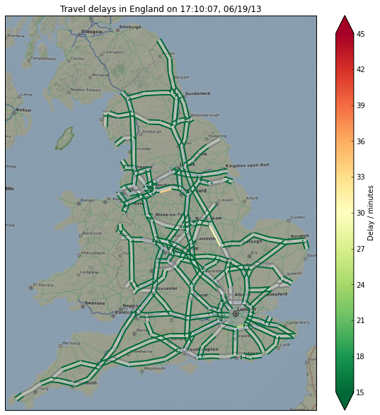
You can see at the current time of writing, the road network of the UK is in a pretty good state.